Change-point baselines and M&V: forecast, backcast, chaining and bills
Workbook exercise mv-baselines · PNNL re-tuning chapters 4 and 10 · about 90 minutes
Goal
Re-tuning is only finished when its savings are measured. Build weather-normalized change-point baselines, judge them against the G14 acceptance tiers and SEP's model-validity tests, and measure a saving four ways: a forecast, a backcast, a three-year chain, and a chain across a closure that has to be handled as a non-routine event. Then do it again with nothing but monthly bills, and see what bills can and cannot tell you.
Learn more
Read these first (PNNL, free):
- Chapter 4: Trend Data Collection and Analysis of the re-tuning training, for the whole-building baseline you are about to fit.
- Chapter 10: Re-Tuning Building Controls and Systems, for where measuring the result fits in the re-tuning process.
The M&V standards are cited by section only; CAMBER's M&V page says how each is applied:
- IPMVP (EVO, 2012, Vol. I): Option C (whole facility), and §4.5.3 for the routine and non-routine adjustment terms.
- ASHRAE Guideline 14-2014: its whole-building acceptance criteria and the Annex B savings uncertainty. CAMBER's G14 gate is CV(RMSE) (30 % daily, 15 % monthly), |NMBE| at most 0.5 % and R² at least 0.75.
- DOE SEP 50001 M&V Protocol (2019 Edition 2): §6.2 (forecast, backcast, chaining), §6.4.1 (model validity: the overall F-test, the variables' p-values and an R² of 0.50 or more), §5.3.2 (evidence and approval for an adjustment).
Datasets and licence
cofactor-drammen: hourly energy of 45 public buildings in Drammen, Norway, 2018-2021, each with its own outdoor temperature. Licence CC-BY-4.0 (open; cite it). About 22 MB. See its data issues.valladolid-uva: two university buildings in Valladolid, Spain, hourly electricity 2016-2020. Licence CC-BY-4.0 (open; cite it). About 6 MB. See its data issues.bdg2: the Building Data Genome 2 meters; one Fox lodging building's meters become synthetic bills (below). Licence CC-BY-SA-4.0 (open; cite it). About 270 MB. See its data issues.
The meters used: the COFACTOR main meters b6400_ElImp and b6404_ElImp (two schools) and
b6410_ElImp (a nursing home); UVA_A (Faculty of Science) and UVA_B (Faculty of Economics,
where the publisher describes an equipment replacement); Fox_lodging_Stephen__chilledwater and
Fox_lodging_Stephen__electricity.
The bills are synthetic. No utility issued them: make_bills.py below cuts a real hourly
meter into read-to-read periods of 28 to 35 days, so the bill-only method can be tried on data
anyone can check. Label them synthetic wherever you show them.
Setup
In the lab
- Run
camber laband open the URL it prints (http://127.0.0.1:8765/lab?token=...). - Tick
cofactor-drammen,valladolid-uvaandbdg2and press Fetch & ingest. - Use trends to look at the meters; the M&V runs below use the command line.
On the command line
camber datasets fetch cofactor-drammen
camber datasets fetch valladolid-uva
camber datasets fetch bdg2
camber datasets ingest cofactor-drammen valladolid-uva bdg2 --store lab_store
Part 1, forecast and backcast. The same three COFACTOR meters, 2018 against 2019, once each way. Both configs model each day's energy on its mean outdoor temperature plus an occupied-day driver (weekdays that are not Norwegian public holidays):
camber datasets config cofactor-drammen --exercise mv-baselines--forecast --store lab_store --out fc.json
camber run fc.json --out fc_out
camber datasets config cofactor-drammen --exercise mv-baselines--backcast --store lab_store --out bc.json
camber run bc.json --out bc_out
Part 2, chaining. The two Valladolid buildings: 2016 baseline, 2017 intermediate, 2018 reporting, with an occupied-day driver on Castilla y León's public holidays:
camber datasets config valladolid-uva --exercise mv-baselines --store lab_store --out chain.json
camber run chain.json --out chain_out
Part 3, a chain across a closure. The COFACTOR meters chained 2018, 2019, 2020, with the
spring 2020 school closure entered as a non-routine adjustment (read its ledger entry in
covid.json):
camber datasets config cofactor-drammen --exercise mv-baselines--covid --store lab_store --out covid.json
camber run covid.json --out covid_out
Part 4, bills only. Save this as make_bills.py next to lab_store:
import sys

import pandas as pd
from camber.store import ParquetStore

store, equip, out = sys.argv[1], sys.argv[2], sys.argv[3]
frame = ParquetStore(store).read_role_frame(facility_id="ds-bdg2-fox", equip=equip)
daily = frame.iloc[:, 0].resample("1D").sum(min_count=24)  # NaN unless all 24 hours
lengths = [30, 33, 28, 31, 35, 29, 32]  # read-to-read days, repeating
rows, start, k = [], daily.index[0], 0
while start <= daily.index[-1]:
    end = start + pd.Timedelta(days=lengths[k % len(lengths)] - 1)
    days = daily[start:end]
    if len(days) == (end - start).days + 1 and days.notna().all():  # no missing day
        rows.append({"start": start.date(), "end": end.date(), "energy": round(days.sum(), 1)})
    start, k = end + pd.Timedelta(days=1), k + 1
pd.DataFrame(rows).to_csv(out, index=False)
print(len(rows), "synthetic bills written to", out)
and this as bills.json: the 2016 bills are the baseline, the 2017 bills the reporting period,
and the degree-day bases are chosen from the bills ("base_f": "auto"):
{
  "source": {"kind": "store", "store": "lab_store", "facility_id": "ds-bdg2-fox"},
  "shared_oat": {"equip": "weather", "role": "oat"},
  "rules": [],
  "mv": [{"bills": {"file": "bills.csv", "energy": "energy"}, "name": "synthetic bills",
          "period": ["2016-01-01", "2016-12-31"],
          "reporting_period": ["2017-01-01", "2017-12-31"],
          "method": "forecast", "base_f": "auto", "calendarize": true, "validity": "both"}]
}
Then:
python make_bills.py lab_store Fox_lodging_Stephen__chilledwater bills.csv
camber run bills.json --out bills_out
Repeat the two commands with Fox_lodging_Stephen__electricity for the second meter.
Steps
- Judge the baselines. In
fc_out/findings.json, read each meter'smv_baseline: model form, R², CV(RMSE), NMBE andaccept(the G14 gate). - Forecast. Read each
mv_savings: the avoided energy, its 90 % band (abs_uncertainty),sep_validand the caveats. No energy measure is documented at these buildings in 2019. - Backcast. Compare
bc_outwithfc_out, meter by meter. - Chain. In
chain_out, read both buildings' baselines and their chained savings, SEnPI and caveats. - Across the closure. In
covid_out, comparesavingswithadjusted_savingsand read theadjustmentsentry (itsrate,resolved_amountandmaterial). - Bills. Build both bill files and read
bills_out:n_bills, the chosen bases, R², CV(RMSE) against the monthly tier, themodel_comparisontable and the caveats.
Questions
- Which 2018 COFACTOR baselines meet the G14 gate, and why does
b6404_ElImp's not, although its CV(RMSE) is within the daily tier? What does SEP §6.4.1 say about the same model? - The forecast puts one school's 2019 saving outside its uncertainty band. Which school, how large a saving, and does the backcast agree? What would you do before reporting it?
- Is the nursing home's forecast saving distinguishable from zero?
- In the Valladolid chain, what saving does each building show, and is either baseline acceptable under G14? Under SEP's R² test? What does the chain leave unmodelled?
- What does the closure adjustment do to
b6400_ElImp's chained saving, and why does the unadjusted figure mislead? - For the synthetic chilled-water bills: how many bills make the baseline, which cooling base do the bills choose, and why does a fit with a high R² still fail the monthly G14 tier?
- For the synthetic electricity bills: what does R² say, and why is the model not SEP-valid? Is the forecast saving meaningful?
What CAMBER shows
mv_baseline:modelandmodel_form,r2,cv_rmse,nmbe,accept,rho; for bills alson_bills,n_days,heating_base_f/cooling_base_f,base_selection,model_comparisonandcalendarized.mv_savings:method,basis,kernel, the saving andsavings_pct,abs_uncertaintyat 90 %,coverage_tier,enpi(the SEnPI),sep_validwithsep_validity; for a chain the intermediate model; with a ledgeradjusted_*,adjustmentsand thewaterfall.- Caveats on every finding: they say when a saving is "for information only", when a model is not SEP-valid and why, and when the band is optimistic.
camber mv reportdraws the same results as an HTML page (see M&V).
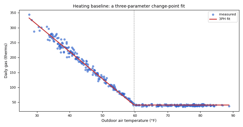
Synthetic illustration, not this exercise's dataset: a daily heating baseline fitted with best_model. Gas use falls with outdoor temperature down to a base load above the change point near 60 °F.
Caveats
- A saving with no documented measure behind it is a change to explain, not a saving to claim.
- CAMBER's G14 gate (above) is CAMBER's reading of the guideline; CalTRACK is stricter in other ways (see M&V).
- The occupied-day driver knows public holidays, not school breaks or academic calendars. Both datasets have breaks the driver cannot see.
- A meter-derived non-routine adjustment carries IPMVP's caution about using the same meter for the event and the saving; CAMBER prints it as a caveat.
- The bills are synthetic and whole-day exact: real bills carry estimated reads, meter-read timing and rounding.
- The default kernel is G14's; its caveat says the exact kernel covers better. Try
"kernel": "exact"in the configs.
Going further
- Add
"kernel": "exact"tofc.jsonand compare the bands. - Replace the chain's occupied-day driver with an explicit academic calendar
(
break_calendar, see M&V) and re-run part 2. - Version the forecast baseline: add
"mv_store": "mv_baselines.json"tofc.json, runcamber mv freeze fc.json --reason "2018 baseline"(a dry run; add--applyto write), thencamber mv run fc.jsonandcamber mv report fc.json --out mv.html.